![]()
A variety of latent Markov models
(Mews,
Koslik, and Langrock 2024), including hidden Markov
models (HMMs), hidden semi-Markov models
(HSMMs), state-space models (SSMs) and
continuous-time variants can be formulated and
estimated within the same framework via directly maximising the
likelihood function using the so-called forward
algorithm
(Zucchini,
MacDonald, and Langrock 2016). Applied researchers often need custom
models that standard software does not easily support. Writing tailored
R code offers flexibility but suffers from slow estimation
speeds. This R package solves these issues by providing
easy-to-use functions (written in C++ for speed) for common tasks like
the forward algorithm. These functions can be combined into custom
models in a Lego-type approach, offering up to 10-20 times faster
estimation via standard numerical optimisers. In its most recent
iteration, LaMa allows for automatic differentiation with
the RTMB package which drastically increases speed and
accuracy even more.
The most important families of functions are
the forward family that calculates the
log-likelihood for various different models,
the tpm family for calculating transition
probability matrices,
the stationary family to compute stationary and
periodically stationary distributions
as well as the stateprobs and viterbi
families for local and global decoding.
You can install the released package version from CRAN with:
install.packages("LaMa")or the development version from Github:
remotes::install_github("janoleko/LaMa")To aid in building fully custom likelihood functions, this package contains several vignettes that demonstrate how to simulate data from and estimate a wide range of models using the functions included in this package.
HMMs, from simple to complex:
Other latent Markov model classes:
We analyse the trex data set contained in the package.
It contains hourly step lengths of a Tyrannosaurus rex, living 66
million years ago. To these data, we fit a simple 2-state HMM with
state-dependent gamma distributions for the step lengths.
library(LaMa)
#> Loading required package: RTMB

head(trex, 3)
#>   tod      step     angle state
#> 1   9 0.3252437        NA     1
#> 2  10 0.2458265  2.234562     1
#> 3  11 0.2173252 -2.262418     1
We start by defining the negative log-likelihood function. This is
made really convenient by the functions tpm() which
computes the transition probability matrix via the multinomial logit
link, stationary() which computes the stationary
distribution of the Markov chain and forward() which
calculates the log-likelihood via the forward algorithm.
nll = function(par, step){
  # parameter transformations for unconstrained optimisation
  Gamma = tpm(par[1:2]) # rowwise softmax
  delta = stationary(Gamma) # stationary distribution
  mu = exp(par[3:4]) # state-dependent means
  sigma = exp(par[5:6]) # state-dependent sds
  # calculating all state-dependent probabilities
  allprobs = matrix(1, length(step), 2)
  ind = which(!is.na(step))
  for(j in 1:2) allprobs[ind,j] = dgamma2(step[ind], mu[j], sigma[j])
  # simple forward algorithm to calculate log-likelihood
  -forward(delta, Gamma, allprobs)
}
To fit the model, we define the intial parameter vector and
numerically optimise the above function using nlm():
par = c(-2,-2,             # initial tpm params (logit-scale)
        log(c(0.3, 2.5)),  # initial means for step length (log-transformed)
        log(c(0.2, 1.5)))  # initial sds for step length (log-transformed)

system.time(
  mod <- nlm(nll, par, step = trex$step)
)
#>    user  system elapsed
#>   0.368   0.010   0.380
Really fast for 10.000 data points!
After tranforming the working (unconstrained) parameters to natural
parameters using tpm() and stationary(), we
can visualise the results:
# transform parameters to working
(Gamma = tpm(mod$estimate[1:2]))
#> S1 S2
#> S1 0.8269546 0.1730454
#> S2 0.1608470 0.8391530
(delta = stationary(Gamma)) # stationary HMM
#> S1 S2
#> 0.481733 0.518267
(mu = exp(mod$estimate[3:4]))
#> [1] 0.3034926 2.5057053
(sigma = exp(mod$estimate[5:6]))
#> [1] 0.2015258 1.4908153
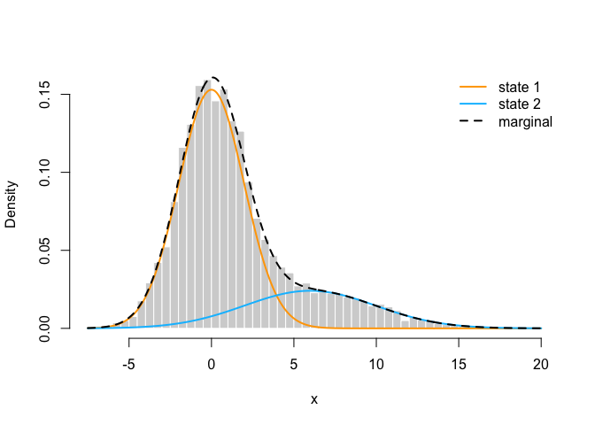
hist(trex$step, prob = TRUE, bor = "white", breaks = 40, main = "", xlab = "step length")
curve(delta[1] * dgamma2(x, mu[1], sigma[1]), add = TRUE, lwd = 2, col = "orange", n=500)
curve(delta[2] * dgamma2(x, mu[2], sigma[2]), add = TRUE, lwd = 2, col = "deepskyblue", n=500)
legend("topright", col = c("orange", "deepskyblue"), lwd = 2, bty = "n", legend = c("state 1", "state 2"))